Quantum #7 - Grover

Jan 2, 2020 Quantum

This is the seventh post of a series of posts about Quantum Computing with Qiskit. The area is very new and the SDK is changing constantly, but hopefully, the series can help you learn a bit about quantum and help me reinforce a couple concepts.

The goal of this post is to discuss Grover’s algorithm. It is an algorithm to solve unstructured search in \(O(\sqrt N)\), which is a quadratic speedup over the classical \(O(N)\) solution.

Unstructured Search

Imagine that you have a hard problem to solve such that your best-known solutions is to try all the possibilities. That problem could be:

Checking if two molecules are identical, i.e. solving graph isomorphism
Finding the shortest route that passes through all cities, the travelling salesman problem

Classically, those are examples of unstructured search problems: the search space (i.e. possible solutions) has so little structure that the best strategy is just to try all possibilities.

The complexity of solving that problem depends on how big the search space is: if there are \(N\) elements to check, the algorithm needs to make \(O(N)\) to an oracle (i.e. the entity that verifies if a solution is valid). That is the best that can be done.

The quantum algorithm that will discuss today goes beyond: it can find the solution with \(O(\sqrt N)\) checks. Considering that there is no structure in the search space, Grover’s algorithm provides an impressive speedup. Moreover, unlike the last two quantum algorithms we discussed, an unstructured search is the component of many real-world problems. Thus, Grover’s algorithm has immediate applications.

For our discussion today, we will pick a specific flavor of the search problem: we will try to find a needle in a haystack.

Needle in a haystack

Imagine that you have a search space with \(N\) elements, with \(N-1\) straws that are useless, and exactly one needle that we are looking for.

Mathematically, the problem is described by a function \(f\):

\[ f(x) = 1 \iff x = s \]

\[ f(x) = 0 \iff x \neq s \]

In which \(s\) is the solution string, i.e. the needle. Notice that \(f\) needs to be implemented by a quantum circuit, that we will call quantum oracle.

Steps of the algorithm

Now that we know the problem Grover’s algorithm solves, it is time to discuss it.

Assumptions

On this discussion, we will assume two things that might not always be true in a search problem:

\(N = 2^{n}\), that is \(N\) is a power of two
There is exactly one solution

Those assumptions are to simplify the discussion. Even though they are not always true, it is not hard to make a problem respect them.

For the first assumption, if we are given a \(M\) that is not a power of two, we can just augment the search space to a \(N\) that is a power of two and have :

\[ x > M \implies f(x) = 0 \]

For the second assumption, Grover’s algorithm can still find a solution when there is multiple: it is just the number of iterations \(K\) that will change.

Step 1

Generate the superposition state:

\[ |\psi\rangle = \frac{1}{\sqrt 2 ^ {n}}\sum_{x \in \{0, 1\}^{n}}|x\rangle \]

And initialize the ancilla qubit to \(\frac{|0\rangle - |1\rangle}{\sqrt 2}\).

Notice that on this step, each possible state \(x\) will have an equal probability of measurement, which is basically guessing the solution. The critical insight from Grover’s algorithm comes on the next step, in which we will try to improve the chance of measuring the solution.

Step 2

Apply Grover’s iteration \(K\) times:

Query the oracle. This is sometimes also called reflection around the solution.
Invert about the mean. This is sometimes also called reflection around the superposition state.

The value \(K\) is given by \(K \approx \frac{\pi \sqrt N}{4}\). Thus, the algorithm makes \(O(\sqrt N)\) queries to the oracle.

Step 3

Measure the qubits. \(s\) will be the measurement with a high probability. A lower-bound for correctness is:

\[ P = 1 - \frac{1}{N} \]

Hence, for very big \(N\) our algorithm will guess the solution with a very high chance.

Grover’s iteration

At each iteration, Grover’s algorithm has a goal: to increase the amplitude \(\alpha_{s}\) of the solution and to decrease the amplitude \(\alpha_{x}\) of the non-solutions. To achieve it, it performs two specific steps as we will discuss.

Phase kickback

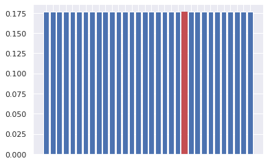
Consider that at an arbitrary iteration of the algorithm, we will have a state \(|\psi\rangle\):

\[ |\psi\rangle = \sum_{x \in \{0, 1\}^{n}}\alpha_{x} |x\rangle \]

Graphically, the amplitudes could be seen as:

The first step of the Grover iteration is to query the oracle. The oracle will be a transformation \(|x\rangle|a\rangle \rightarrow |x\rangle|a \oplus f(x)\rangle\).

We will now reuse a trick that was first discussed in Deutsch-Jozsa’s algorithm: because the ancilla is \(\frac{|0\rangle - |1\rangle}{\sqrt 2}\), then the phase will kickback in the form of a coefficient \((-1)^{f(x)}\), and the ancilla will remain unchanged.

Hence, that yields:

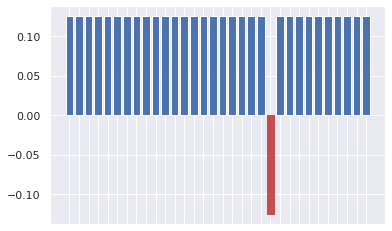
\[ U_{\omega}|\psi\rangle = \sum_{x \in \{0, 1\}^{n}} (-1)^{f(x)} \alpha_{x} |x\rangle \]

Notice that this time, only one amplitude is negative: that of the solution. Graphically, it can be seen as:

The next step is to perform an inversion about the mean. The idea is that combining phase kickback with a mean inversion, we will make the amplitude of the solution grow while reducing the amplitude of nonsolutions.

Inversion about the mean

An inversion about the mean is reflecting the terms of a sequence \(C\) according to the mean \(\overline{C}\). That is, we will find a new sequence \(D\) such that each term is \(C_{i}\) reflected.

Imagine that you have an element \(C_{i}\). We will find a new element \(D_{i}\) such that the distance between \(D_{i}\) and \(\overline{C}\) is the same as the distance between \(C_{i}\) and \(\overline{C}\). Mathematically, that can be written as:

\[ |D_{i} - \overline{C}| = |C_{i} - \overline{C}| \]

Solving the equation and ignoring the case in which \(C_{i} = D_{i}\), we obtain:

\[ D_{i} = 2\overline{C} - C_{i} \]

After the mean inversion transformation, \(\overline{D} = \overline{C}\) holds as well.

At this point, you might be asking: what does mean inversion has to do with quantum computing? To answer that question, an example will do. Suppose that we have the sequence \(\{1, 1, 1, 1\}\) and we flip the sign of the third 1, that is we have:

\[ C = \{1, 1, -1, 1\} \]

The mean of this sequence is \(\frac{1}{2}\). Now if we compute mean inversion using the formula given before, we obtain:

\[ D = \{0, 0, 2, 0\} \]

Something very interesting occurred: during the inversion, the only negative value of the sequence became the most positive while the old positives values diminished.

Hence, mean inversion combined with phase kickback is exactly what we were looking for: it is going to make \(\alpha_{s}\) increase and decrease \(\alpha_{x}\) of the nonsolutions.

Continuing the amplitude visualization we had before, mean inversion yields:

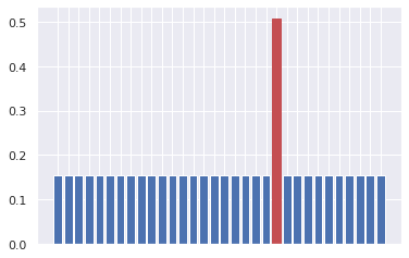
Therefore, the idea is to perform phase kickback and mean inversion until \(\alpha_{s}\) is maximized. We will not discuss the math behind, but it turns out that \(\frac{\pi \sqrt N}{4}\) iterations suffice.

Implementing the quantum oracle

In real applications, the oracle would be a circuit that performs a meaningful computation: it could be solving the travelling salesman problem, trying to break an encryption key or just solving a hard problem in general.

For this example problem, we will emulate a real-world problem: we will have a function that has one value \(s\) such that \(f(s) = 1\) and that \(f(x) = 0\) for all other \(x\).

Classically, it would look like:

def f(x):
    if x == s:
        return 1
    else:
        return 0

The question now is: how does a quantum computer check that the state \(x\) is equal to \(s\)? The answer is: we verify if the binary representation of \(x\) is identical to the binary representation of \(s\).

To do so, we use a multi-qubit Toffoli gate: we AND the equality of each bit. Because of the AND property, \(f(x) = 1\) if and only if each bit of \(x\) is equal to \(s\), otherwise \(f(x) = 0\). That implements exactly what we were looking for.

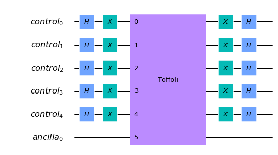
A factor to consider is that if a bit is 0, we need to NOT it so when the AND is done the result is 1. Hence, the circuit implementing \(f\) for a string \(s\) looks like:

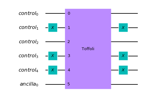
Notice that after applying the Toffoli, we do not want to change \(|x\rangle\) hence we apply NOT again on what was NOTed before.

Implementing inversion about mean

To implement inversion about the mean, we will use the Grover diffusion operator. I will not discuss it much, but the operator can be written as:

\[ \mathcal{D} = -H^{\otimes n}U_{s}H^{\otimes n} \]

The idea is to implement the formula \(2\overline{C} - C_{i}\) using matrix multiplication. It can be shown that \(\mathcal{D} = 2|+\rangle\langle+| - I\), which is the matrix equivalent of the formula we found for mean inversion.

An element of \(\mathcal{D}\) we have not discussed yet is \(U_{s}\): it is similar to the oracle \(U_{\omega}\). It implements a function \(g(x)\) such that \(g(000...0) = 1\) and \(g(x) = 0\) for all other \(x\).

Therefore, we also use a multi-qubit Toffoli gate to implement \(U_{s}\) which yields the following circuit for \(\mathcal{D}\):

Implementing Grover’s algorithm

We can verify that Grover’s algorithm works using Qiskit and running an experiment: in the Jupyter notebook below, we try to find a needle in a haystack.

quantum