This is the fifth post of a series of posts about Quantum Computing with Qiskit. The area is very new and the SDK is changing constantly, but hopefully, the series can help you learn a bit about quantum and help me reinforce a couple concepts.

The goal of this post is to continue the discussion of the Deutsch-Jozsa algorithm, starting off where we stopped on part 1.

Deutsch-Jozsa problem

After having introduced the Deutsch problem, we will now introduce the Deutsch-Jozsa which is a generalization of the Deutsch problem. In particular, the Deutsch problem is the case of Deutsch-Jozsa with \(n = 1\).

Imagine that you have a black box that implements a function from n-bit strings (e.g. 11010) to 0 or 1, that is \(f : \{0, 1 \}^{n} \rightarrow \{0, 1\}\). It is guaranteed that \(f\) is either a balanced or a constant function. You can make a query to the black box with a value \(v\), and the black box will return \(f(v)\). How many queries are needed to decide if the function is constant or balanced?

Just remembering definitions, a function is balanced when the number of values that have \(f(v) = 0\) is equal to the number of values that have \(f(v) = 1\).

This time, we have way more than 4 possible functions, more precisely \(2(\binom{2^{n}}{2^{n-1}} + 1)\). Our classical strategy also needs more queries to classify the function. To deterministically determine the type of the function, we need \(O(2^{n})\) queries because the worst case is when we obtain \(2^{n-1}\) of 0s (or 1, it is symmetric) and still need an additional query to distinguish between balanced or constant.

From a perspective using classical computers, that is (deterministically) the best we can do. A question that arises is: can quantum computers do better? It can be shown that yes, they can. And the speedup is impressive.

Generalazing the solution for multiple bits

We now need to try to generalize our solution from \(n = 1\) to larger values of \(n\). It is worth trying the same solution but now using multiple bits, i.e. to apply a Hadamard to every qubit to generate all possible values, evaluate using the black box, and lastly apply Hadamard gates before measuring. The circuit we obtain looks like:

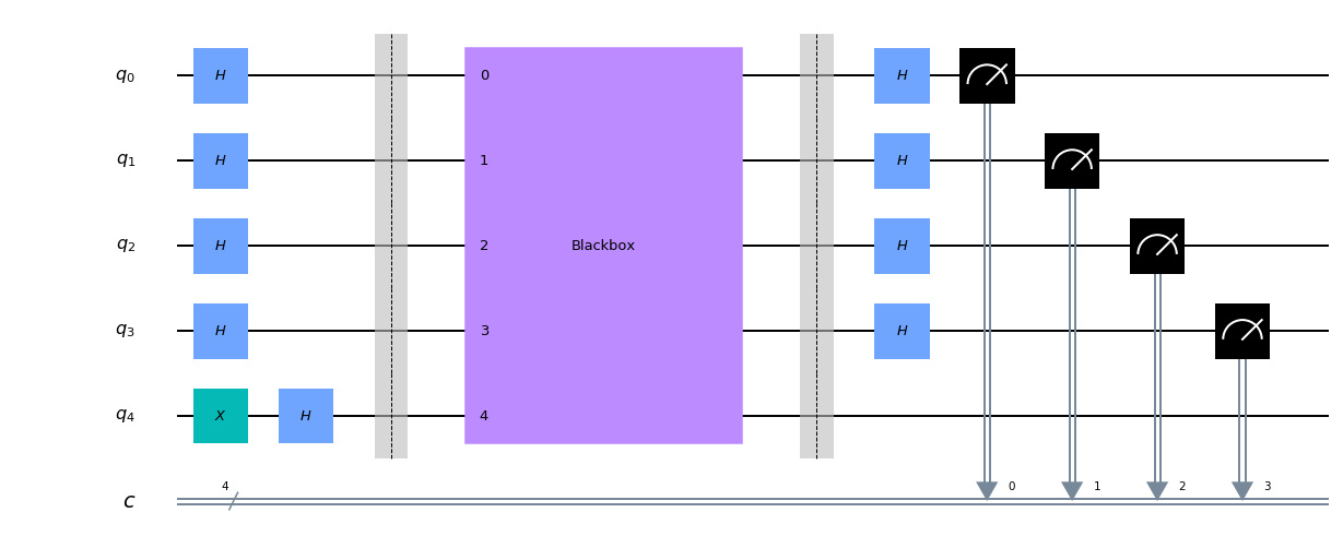
We now need to decide if the circuit provides criteria similar to the previous solution to differentiate between. It is helpful to expand the math to analyze that. After applying the Hadamard gates we have:

\[ |\psi\rangle = |00...0\rangle|0\rangle \rightarrow H^{\otimes N}|\psi\rangle \otimes (\frac{|0\rangle - |1\rangle}{\sqrt 2}) \]

\[ \rightarrow \frac{1}{\sqrt 2 ^ {n}}\sum_{x \in \{0, 1\}^{n}} |x\rangle \otimes (\frac{|0\rangle - |1\rangle}{\sqrt 2}) \]

We then send the input to the blackbox, that yields:

\[ \rightarrow \frac{1}{\sqrt 2 ^ {n}}\sum_{x \in \{0, 1\}^{n}} |x\rangle \otimes (\frac{|0 \oplus f(x)\rangle - |1 \oplus f(x)\rangle}{\sqrt 2}) \]

\[ \rightarrow \frac{1}{\sqrt 2 ^ {n}}\sum_{x \in \{0, 1\}^{n}} (-1)^{f(x)}|x\rangle \otimes (\frac{|0\rangle - |1\rangle}{\sqrt 2}) \]

Like in the last analysis, we used the identity \(|0 \oplus a \rangle - |1 \oplus a \rangle = (-1)^{a}(|0\rangle - |1\rangle)\). We also obtained a similar result: the last qubit does not change, so measuring it is useless and we will not worry about it afterwards.

Given that now we have a mathematical expression representing the state of the qubits, we can analyse the two possible cases before measuring.

Constant case

If \(f\) is constant, then all the \(x\) in the sum before will have the same sign, which can be summarized as:

\[ |\psi\rangle = \pm \frac{1}{\sqrt 2 ^ {n}}\sum_{x \in \{0, 1\}^{n}} |x\rangle \]

Notice that multiplying the whole expression by -1 does not affect the measurements because it is a global phase change. The state that happens on the balanced case after applying the black box is then:

\[ |\psi\rangle = (\frac{|0\rangle + |1\rangle}{\sqrt 2})^{\otimes n} \]

Notice that when we apply the Hadamard gates before measuring, each \(\frac{|0\rangle + |1\rangle}{\sqrt 2}\) becomes \(|0\rangle\) and therefore the final state is \(|00...0\rangle\).

Hence, we are sure that if \(f\) is constant then all measurements will always be 0.

Balanced case

We now need to analyse the other case, when there is no guarantee that all \(|x\rangle\) will have the same sign. Indeed, we do not know anything about \(f\) (just that the number of 0s and 1s is the same) so it is difficult to know the exact probability of an arbitrary state \(|x\rangle\).

One thing we know though is that \(|00...0\rangle\) is always the output of the other case, i.e. the constant case. We may then ask: what is the probability that this case, the balanced case, will output \(|00...0\rangle\)?

To analyze that we need to calculate the coefficient \(\alpha\) of \(|\psi\rangle = \alpha|00...0\rangle + ...\) after applying all the Hadamard gates, which can be seen as multiplying by \(H^{\otimes n}\).

One key property of \(H^{\otimes n}\) is that the first line, the line that will give the \(\alpha\) of the final \(|\psi\rangle\), has constant terms i.e. they are equal. More exactly, all terms of the first line of \(H^{\otimes n}\) are \((\sqrt 2) ^ {-n}\). This fact can be shown by induction and I will just use it, not prove it.

Given that all terms of the first line are \((\sqrt 2) ^ {-n}\), the \(\alpha\) we obtain is:

\[ \alpha = \frac{1}{\sqrt 2 ^ {n}} \frac{1}{\sqrt 2 ^ {n}} \sum_{x \in \{0, 1\}^{n}} (-1)^{f(x)} \]

Now the fact that the function is balanced becomes crucial. Because the number of \(f(x) = 0\) and \(f(x) = 1\) are equal, the sum above is zero! Hence, \(\alpha\) is zero and therefore there is no \(|00...0\rangle\) component in the final state. Because of that, we are guaranteed that not all measurements will be 0, which means that at least one of the measurements will be 1.

Thus, the circuit we used provides criteria to classify \(f\):

• If all the measurements are 0, then \(f\) is constant
• If at least one of the measurements is 1, then \(f\) is balanced

The problem has been solved! The most impressive fact is that only 1 query was used, instead of \(O(2^{n})\) queries. That is an exponential speedup.

Implementing the Deutsch-Jozsa algorithm

We can verify that the Deutsch-Jozsa algorithm works using Qiskit and running an experiment: in the Jupyter notebook below, we try three cases for the black box and verify that our algorithm predicts correctly that it is balanced or constant.

So what?

You might ask: what is the point of the Deutsch-Jozsa algorithm? The algorithm solves a very artificial and useless problem. It has very little practical applications.

The algorithm, in my personal opinion, exemplifies the beauty of quantum computing: it provides an exponential speedup! Not only the speedup is impressive, but it is also unachievable by classical computers. It is one of the first algorithms from a yet-to-be-explored field.

It also exemplifies the less beautiful aspects of it. As of now, quantum computing… is useless. The Deutsch-Jozsa problem is a toy problem to show that two complexity classes for algorithms are different, and that is it. No applications. Not to mention that with Noisy Quantum Computers even running simple algorithms like Deutsch-Jozsa can have errors (qubits and gates are still not perfect).

However, the algorithm still has historical importance and inspired other algorithms that have more practical applications, like Shor’s algorithm for factorizing numbers. Hence, it is still important to study the problem.

A randomized approach

In the initial discussion, we highlighted the deterministic factor. As a side note, we can have a probabilistic algorithm that solves the problem most of the time with an error rate \(\epsilon\). If \(k\) queries are made to the black box, \(\epsilon = 2^{-(k - 1)}\). Because the decrease in \(\epsilon\) is exponential, with a constant and small value of \(k\) we can classify with great confidence. Below is Python code implementing that idea (\(f\) is the function, \(n\) is the number of bits and \(k\) is the number of tries before we stop).

from random import randint

def balanced_or_constant(f, n, k):

    first_guess = f(randint(0, 2**n - 1))

    for i in range(k-1):
        guess = f(randint(0, 2**n - 1))
        if guess != first_guess:
            return "balanced"

    return "constant"