This is the sixth post of a series of posts about Quantum Computing with Qiskit. The area is very new and the SDK is changing constantly, but hopefully, the series can help you learn a bit about quantum and help me reinforce a couple concepts.

The goal of this post is to discuss how to discover a hidden string in a black box using Bernstein-Vazirani’s algorithm. There is also a connection between this algorithm and Deutsch-Jozsa’s algorithm, which was discussed in the last post.

Decoding a hidden string

Imagine that you have a black box (or oracle) that implements a hidden function that takes n-bit strings and returns 0 or 1, that is \(f: \{0, 1\}^{n} \rightarrow \{0, 1\}\). The output of the function is determined by a hidden string \(s\), following the expression:

\[ f(x) = s \cdot x \mod 2 \]

How many queries are needed to discover \(s\)?

To clarify the notation used, by \(s \cdot x\) we mean the bitwise dot product of \(s\) and \(x\). Mathematically, if \(s = a_{0}a_{1}a_{2}...a_{n-1}\) and \(x = b_{0}b_{1}b_{2}...b_{n-1}\) then we define:

\[ s \cdot x = \sum_{0}^{n-1} a_{i}b_{i} \]

From now on in the post, I will also write \(s \cdot x\) instead of \(s \cdot x \mod 2\) for convenience. Some authors even define \(s \cdot x\) as the sum mod 2.

Classical approach

Before discussing the quantum solution to the problem, it is important to understand the classical solution. We can interpret \(f\) as a function that computes the bitwise AND of \(s\) and \(x\), and then counts the parity of turned on bits on \(s \wedge x\).

Hence, when we are trying to discover \(s\) by evaluating \(f(x)\), it is never advantageous to have \(x\) with many bits turned on because we only obtain the parity of it.

A good strategy then is to use \(x\) with only one bit set on, that is \(x \in \{100..., 010..., 001.., ...\}\). The Python code below implements exactly that idea:

def guess_hidden_string(f, n):

    s = 0

    for i in range(n):
        result = f(2**i)
        if result == 1:
            s += 2**i

    return s

This approach needs n queries to discover the n-bit hidden string, and overall \(O(n)\) is the best we can achieve with classical computers. Can quantum computers do better?

Implementing the quantum oracle

Before we try to find a quantum solution, we will briefly discuss how to implement the quantum oracle because that step is needed to implement the actual algorithm.

One key fact when implementing the oracle was discussed in the section before: \(f\) can be interpreted as discussing the parity of set bits of the bitwise AND. Hence, we may write:

\[ f(x) = (\sum_{0}^{n-1} a_{i} \wedge b_{i}) \mod 2 \]

Recalling that the XOR operator (\(\oplus\)) can be seen as the plus operator mod 2, we can go even further and write:

\[ f(x) = (a_{0} \wedge b_{0}) \oplus (a_{1} \wedge b_{1}) \oplus ... \oplus (a_{n-1} \wedge b_{n-1}) \]

The XOR operator is represented by the CNOT gate on quantum computing, because it takes \(|a\rangle\) to \(|a \oplus b\rangle\). Thus, our quantum oracle looks like the following:

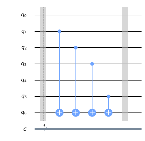
For every bit \(a_{i} = 1\) in \(s\), we apply the CNOT gate from the i-th qubit to the working qubit. That happens because if \(a_{i} = 0\), then \(a_{i} \wedge b_{i} = 0\) and \(x \oplus 0 = x\) thus we can ignore it. CNOT gates are used because they are the equivalent of \(\oplus\), as discussed before.

Bernstein-Vazirani

This time, we will start by giving the solution to the problem. We will very computationally that it works and then justify it mathematically.

The following circuit guesses the hidden string:

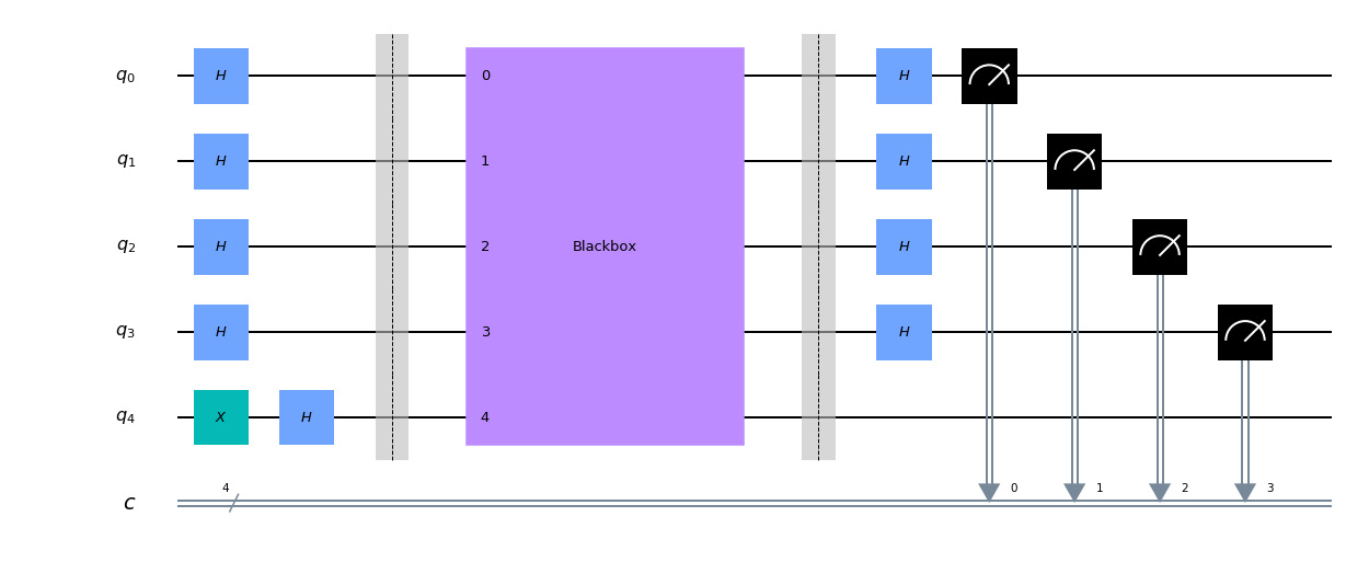
Firstly, we change the working qubit from \(|0\rangle\) to \(|1\rangle\) by using the X gate.

Secondly, we apply Hadamard gates to the n qubits. That state is then given to the quantum oracle.

In the next step, the oracle yields the \(f(x)\) for the working qubit of each state, and that qubit is discarded afterward.

To conclude the algorithm, we apply Hadamard gates again and measure the qubits. It is guaranteed that 100% of the measurements will be \(s\), the hidden string we were looking for. We will analyze later why \(|s\rangle\) is the state that originates after querying the oracle.

Notice that we discovered the hidden string using only one query to the oracle, compared to the \(O(n)\) queries required by the classical algorithm.

Implementing the Bernstein-Vazirani algorithm

We can verify that the Bernstein-Vazirani algorithm works using Qiskit and running an experiment: in the Jupyter notebook below, we try to guess a hidden string from a black box.

Analysis: why the circuit works

The first step in the analysis is to notice that the circuit used in Bernstein-Vazirani’s algorithm is identical to the circuit in Deutsch-Jozsa’s algorithm. That is surprising at first because one algorithm works to find a hidden string and the other to distinguish between balanced and constant functions.

Now, we will use a result from the discussion on the last post, to remember that the state after querying the oracle is:

\[ |\psi\rangle = \frac{1}{\sqrt 2 ^ {n}}\sum_{x \in \{0, 1\}^{n}} (-1)^{f(x)}|x\rangle \]

But this time, we know that our oracle is described by \(f(x) = s \cdot x\). Thus:

\[ |\psi\rangle = \frac{1}{\sqrt 2 ^ {n}}\sum_{x \in \{0, 1\}^{n}} (-1)^{s \cdot x}|x\rangle \]

We will now claim that:

\[ H^{\otimes n} |\psi\rangle = |s\rangle \]

That is, that applying the Hadamard gate to each qubit takes us from \(|\psi\rangle\) to \(|s\rangle\).

To prove so, we will work backwards. Because \(H\) is the inverse gate of itself, then \(H^{\otimes n}\) is the inverse of \(H^{\otimes n}\). Thus, proving our claim is equivalent to showing that:

\[ H^{\otimes n} |s\rangle = \frac{1}{\sqrt 2 ^ {n}}\sum_{x \in \{0, 1\}^{n}} (-1)^{s \cdot x}|x\rangle \]

It would be useful to find a formula for \(H^{\otimes n} |s\rangle\) . We can start by finding a formula for \(H\), that is:

\[ H |a\rangle = \frac{|0\rangle + (-1)^{a}|1\rangle}{\sqrt 2} \]

The identity can be proved by verification of \(a = 0\) and \(a = 1\). We can even go further and write:

\[ H |a\rangle = \frac{1}{\sqrt 2} \sum_{b \in \{0, 1\}} (-1)^{ab}|b\rangle \]

Now that we have an identity for \(n = 1\), it would be useful to generalize for greater values of n. For \(n = 2\), we can think of the multiple qubits as tensor products and thus:

\[ H^{\otimes 2}|a,c\rangle = (\frac{1}{\sqrt 2} \sum_{b \in \{0, 1\}} (-1)^{ab}|b\rangle) \otimes (\frac{1}{\sqrt 2} \sum_{d \in \{0, 1\}} (-1)^{cd}|c\rangle) \]

We may rewrite it in a formula closer to the \(s \cdot x\) product we defined earlier, that is:

\[ H^{\otimes 2}|s\rangle = \frac{1}{(\sqrt 2)^{2}} \sum_{x \in \{0, 1\}^{2}} (-1)^{s_{0}x_{0} + s_{1}x_{1}}|x\rangle \]

Because of the cycle of powers of -1, \((-1)^{a} = (-1)^{a \mod 2}\) and thus the -1 exponent is \(s \cdot x\)! Therefore, we may generalize to all \(n\) (the proof can be done by induction):

\[ H^{\otimes n}|s\rangle = \frac{1}{(\sqrt 2)^{n}} \sum_{x \in \{0, 1\}^{n}} (-1)^{s\cdot x}|x\rangle \]

Hence, our circuit works because it takes \(|\psi\rangle\) to \(|s\rangle\) due to the inverse nature of \(H^{\otimes n}\).

The connection between Deutsch-Jozsa’s and Bernstein-Vazirani’s algorithm becomes clearer then:

• \(f(x) = s \cdot x\) is a balanced function (or constant if \(s\) is all zeroes)!
• If a black box from Deutsch-Jozsa’s returns a state \(|s\rangle\) with 100% chance, then the black box implements \(f(x) = s \cdot x\)