Quantum #1 - Basic Quantum Computing

This is the first post of a series of posts about Quantum Computing with Qiskit. The area is very new and the SDK is changing constantly, but hopefully, the series can help you learn a bit about quantum and help me reinforce a couple concepts.

The goal of this post is to introduce a more hands-on approach to quantum computing using Qiskit. For a friendly introduction to quantum computing in general, I recommend the essay Quantum computing for the very curious by Matuschak and Nielsen.

The qubit

Quantum computers are made of qubits like classical computers are made of bits. However, qubits vectors and thus they have components. There are two very important qubits \(|0\rangle\) and \(|1\rangle\) that relate to their classical 0 and 1 counterparts. In vector notation, they are:

\[ |0\rangle = \begin{bmatrix}1 \\ 0\end{bmatrix} \]

\[ |1\rangle = \begin{bmatrix}0 \\ 1\end{bmatrix} \]

In general, every qubit \(|\psi\rangle\) has a \(|0\rangle\) component and a \(|1\rangle\) component, that is:

\[ |\psi\rangle = \alpha|0\rangle + \beta|1\rangle \]

We can also write that superposition (or linear combination) in the matrix form.

\[ |\psi\rangle = \begin{bmatrix}\alpha \\ \beta\end{bmatrix} \]

It is important to remember that \(\alpha\) and \(\beta\) may be complex numbers! Thus, the imaginary number \(i\) may appear in the components. For example, following qubit is valid:

\[ |\psi\rangle = \begin{bmatrix}\frac{1 + i}{\sqrt 2} \\ 0\end{bmatrix} \]

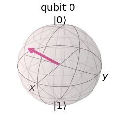
Lastly, one key factor for qubits is that they are unitary vectors that is:

\[ || |\psi\rangle || = 1 \]

Thus, we may visualize a qubit as a 3d vector in a sphere of radius 1:

Quantum gates & Quantum Circuits

A quantum circuit is a collection of qubits and classical bits. The building blocks of quantum circuits are quantum gates: they modify qubits and allow quantum computing to achieve arbitrary qubit states as we discussed before.

In Qiskit, a quantum circuit can be initialized by:

from qiskit import *
circuit = QuantumCircuit(n_qubits, n_classical_bits)

In general, a gate \(U\) can be added to a circuit by:

circuit.u(target_qubit)

A fact to notice is that there is an infinite number of qubit gates! A gate is any device that takes a qubit \(|\psi\rangle\) and outputs another valid qubit \(|\phi\rangle\). In general, we have that a gate \(U\) can be represented by a matrix:

\[ U = \begin{bmatrix} a & b \\ c & d\end{bmatrix} \]

By applying the gate \(U\) to a qubit \(|\psi\rangle = \alpha|0\rangle + \beta|1\rangle\), we obtain:

\[ |\phi\rangle = U|\psi\rangle = (a\cdot\alpha + b\cdot\beta)|0\rangle + (c\cdot\alpha + d\cdot\beta)|1\rangle \]

Notice that \(U\) must preserve the length of \(|\psi\rangle\) in order for \(|\phi\rangle\) to be a valid qubit! Thus \(U\) is a special type of matrix called a unitary matrix. Mathematically:

\[ UU^{\dagger} = I \]

Where \(U^{\dagger}\) is the conjugate transpose. It is important to see that \(U^{\dagger}\) can undo the transformation from \(U\): it takes \(|\phi\rangle\) to \(|\psi\rangle\).

Because of the matrix multiplication property of the gates, applying multiple quantum gates such as \(U_{a}\) and then \(U_{b}\) is equivalent to applying a gate \(G\) such that:

\[ G = U_{a}U_{b} \]

It is important to notice that gate composition also implies gate decomposition. The quantum gate you are applying might be a synthesis of other easier to implement gates in real life such that \(G = U_{a}U_{b}U_{c}\).

Even though there is an infinite amount of gates, some are very famous because they are more used than others and have a special place in quantum computing and Qiskit. They are:

The Pauli-X gate

The Pauli-X gate is the quantum equivalent of the NOT gate, that is it takes 0 to 1 and 1 to 0. Mathematically:

\[ |0\rangle \overset{X}{\rightarrow} |1\rangle \]

\[ |1\rangle \overset{X}{\rightarrow} |0\rangle \]

\[ \alpha|0\rangle + \beta|1\rangle \overset{X}{\rightarrow} \beta|0\rangle + \alpha|1\rangle \]

To use the Pauli-X gate in Qiskit, it suffices to write:

circuit.x(target_qubit)

Graphically, the gate is represented as:

Because \(X\) is a gate, it can be written as a matrix as we discussed before:

\[ X = \begin{bmatrix} 0 & 1 \\ 1 & 0\end{bmatrix} \]

An important property of \(X\) is that \(X = X^{\dagger}\), thus \(X\) is the inverse gate of itself! That means that if we apply twice the Pauli-X Gate to a qubit, we will still have the same qubit.

The Pauli-Z gate

The Pauli-Z gate is a quantum gate that leaves the \(|0\rangle\) component intact but flips the sign of the \(|1\rangle\) component. Mathematically:

\[ |0\rangle \overset{Z}{\rightarrow} |0\rangle \]

\[ |1\rangle \overset{Z}{\rightarrow} -|1\rangle \]

\[ \alpha|0\rangle + \beta|1\rangle \overset{Z}{\rightarrow} \alpha|0\rangle - \beta|1\rangle \]

To use the Pauli-Z gate in Qiskit, it suffices to write:

circuit.z(target_qubit)

Graphically, the gate is represented as:

The matrix representation of \(Z\) is:

\[ Z = \begin{bmatrix} 1 & 0 \\ 0 & -1\end{bmatrix} \]

An important property of \(Z\) is that \(Z = Z^{\dagger}\), thus \(Z\) is the inverse gate of itself! That means that if we apply twice the Pauli-Z Gate to a qubit, we will still have the same qubit.

The Pauli-Y gate

The Pauli-Y gate is a gate that has only pure imaginary entries. It is similar to the \(X\) gate but has its entries multiplied by \(i\) and the top term is \(-i\). Mathematically, it acts as follows:

\[ |0\rangle \overset{Y}{\rightarrow} i|1\rangle \]

\[ |1\rangle \overset{Y}{\rightarrow} -i|0\rangle \]

\[ \alpha|0\rangle + \beta|1\rangle \overset{Y}{\rightarrow} -i\beta|0\rangle + i\alpha|1\rangle \]

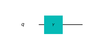
To use the Pauli-Y gate in Qiskit, it suffices to write:

circuit.y(target_qubit)

Graphically, the gate is represented as:

The matrix representation of \(Y\) is:

\[ Y = \begin{bmatrix} 0 & -i \\ i & 0\end{bmatrix} \]

An important property of \(Y\) is that \(Y = Y^{\dagger}\), thus \(Y\) is the inverse gate of itself! That means that if we apply twice the Pauli-Y Gate to a qubit, we will still have the same qubit.

The Hadamard gate

The Hadamard gate is a gate to generate superposition, and it is hard to find a classical equivalent of it: it is a quantum gate by nature. Given \(|0\rangle\), it generates a mix of \(|0\rangle\) and \(|1\rangle\), and does the same for \(|1\rangle\). Mathematically:

\[ |0\rangle \overset{H}{\rightarrow} \frac{|0\rangle + |1\rangle}{\sqrt 2} \]

\[ |1\rangle \overset{H}{\rightarrow} \frac{|0\rangle - |1\rangle}{\sqrt 2} \]

\[ \alpha|0\rangle + \beta|1\rangle \overset{H}{\rightarrow} \frac{(\alpha + \beta)}{\sqrt 2}|0\rangle + \frac{(\alpha - \beta)}{\sqrt 2}|1\rangle \]

Notice that \(\frac{|0\rangle + |1\rangle}{\sqrt 2}\) and \(\frac{|0\rangle - |1\rangle}{\sqrt 2}\) are so important because they can be seen as an alternative basis, that they deserve their own symbols:

\[ |+\rangle= \frac{|0\rangle + |1\rangle}{\sqrt 2} \]

\[ |-\rangle= \frac{|0\rangle - |1\rangle}{\sqrt 2} \]

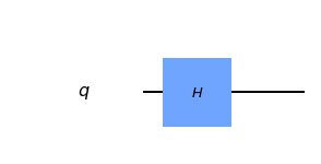
To use the Hadamard gate in Qiskit, it suffices to write:

circuit.h(target_qubit)

Graphically, the gate is represented as:

The matrix reprenstation of the Hadamard gate is:

\[ H = \frac{1}{\sqrt 2}\begin{bmatrix} 1 & 1 \\ 1 & -1\end{bmatrix} \]

An important property of \(H\) is that \(H = H^{\dagger}\), thus \(H\) is the inverse gate of itself! That means that if we apply twice the Hadamard gate to a qubit, we will still have the same qubit.

Executing a circuit in Qiskit

In Qiskit, we need a backend to execute a quantum circuit. That backend might be either a real quantum computer or a simulator. The syntax to run a circuit is:

job = execute(circuit, backend, shots=n_times_to_execute)

There are three key simulators in Qiskit that you must be aware of:

• qasm_simulator: simulates the circuit and performs measurements
• unitary_simulator: simulates the circuit and outputs the unitary matrix that represents it
• statevector_simulator: simulates the circuit and outputs the state of the qubit

The syntax to obtain the specific backend with the simulator we want is:

simulator = Aer.get_backend(backend_name)

Notice that after running the circuit either in a simulator in a real device, we would want the results! The code snippet below describes how to obtain it:

result = job.result()
result.get_unitary()  # if the backend is unitary_simulator
result.get_statevecor() # if the backend  is statevector_simulator

Jupyter notebooks exemplifying the process are given below:

Measurements

Even though qubits are a superposition of \(|0\rangle\) and \(|1\rangle\), when a measurement is made, the output will be either 0 or 1. For a given qubit \(|\psi\rangle = \alpha|0\rangle + \beta|1\rangle\), there is a \(|\alpha^{2}|\) probability that the measurement will be 0 and a \(|\beta^{2}|\) probability that the measurement will be 1.

Because the sum of the probabilities of all events is equal to one, we may write:

\[ |\alpha^{2}| + |\beta^{2}| = 1 \]

In Qiskit, a measurement can be made using the following syntax:

circuit.measure(target_qubit, target_classical_bit)

After executing the job in a real quantum computer or in a simulator, the obtained measurements will be available in a dictionary where the key is the measurement and the value is the count of the measurements:

result = job.result()
measurement_counts = result.get_counts()

In general, it is also useful to visualize the measurements using a histogram. That can be done through:

from qiskit.visualization import plot_histogram
plot_histogram(measurement_counts)

A Jupyter notebook exemplifying the measurement process is given below:

Multiple qubits

So far we have discussed only systems with exactly one qubit! However, quantum circuits are generally composed of multiple qubits. For example, for a two-qubit system, there are four states: \(|00\rangle\), \(|01\rangle\), \(|10\rangle\) and \(|11\rangle\). A 2-qubit system can be described then as:

\[ |\psi\rangle = \alpha|00\rangle + \beta|01\rangle + \gamma|10\rangle + \delta|11\rangle \]

A system of n qubits will have \(2^{n}\) states, hence using the ket notation is more convenient than writing matrices with \(2^{n}\) entries.

For multiple qubit system, it is also common to use the tensor product (\(\otimes\)) to describe the state. If \(|\psi\rangle = \alpha|0\rangle + \beta|1\rangle\) is a single qubit and \(|\phi\rangle\) is a qubit, then we define:

\[ |\psi\rangle \otimes |\phi\rangle = \begin{bmatrix}\alpha|\phi\rangle \\ \beta|\phi\rangle\end{bmatrix} \]

Sometimes also written \(|\psi\rangle|\phi\rangle\). Notice that \(|00\rangle = |0\rangle \otimes |0\rangle\). The same apply for more qubits: \(|011\rangle = |0\rangle \otimes |1\rangle \otimes |1\rangle\).

To make it clearer, an example is useful. If \(|\psi\rangle = \alpha|0\rangle + \beta|1\rangle\) and \(|\phi\rangle = \gamma|0\rangle + \delta|1\rangle\), then:

\[ |\psi\rangle \otimes |\phi\rangle = \alpha\gamma|00\rangle + \alpha\delta|01\rangle + \beta\gamma|10\rangle + \beta\delta|11\rangle \]

One last remark is: not every state can be written as a tensor product of qubits! Those states are called entangled. An example of an entangled state is:

\[ |\Phi^{+}\rangle = \frac{|00\rangle + |11\rangle}{\sqrt 2} \]

Multiple-qubit gates

In the first gate section, we discussed gates that operated on a single qubit. In this section, we will discuss gates that operate on two or more qubits. They are still unitary gates:

\[ UU^{\dagger} = I \]

Their dimensions, however, are different. A gate that operates on n qubits has dimensions of \(2^{n} \times 2^{n}\). It is also relevant to know how to write single-qubit gates for multiple qubit systems: they are written using the tensor product such as \(H \otimes Z\): in this example, we apply the Hadamard gate to the first qubit and the Pauli-Z gate to the second qubit.

Again, there is an infinite number of multiple qubit gates. Some that deserve special attention and have a special place in Qiskit are:

Controlled NOT gate

The Controlled NOT gate applies the NOT gate (Pauli-X gate) to a target qubit based on a control qubit. If the control qubit is 1, then \(X\) is applied to the target. Otherwise, the target is not affected. Mathematically, considering the first qubit as control and the second one as a target:

\[ |00\rangle \overset{CX}\rightarrow |00\rangle \]

\[ |01\rangle \overset{CX}\rightarrow |01\rangle \]

\[ |10\rangle \overset{CX}\rightarrow |11\rangle \]

\[ |11\rangle \overset{CX}\rightarrow |10\rangle \]

\[ \alpha|00\rangle + \beta|01\rangle + \gamma|10\rangle + \delta|11\rangle \overset{CX}\rightarrow \alpha|00\rangle + \beta|01\rangle + \delta|10\rangle + \gamma|11\rangle \]

To use the CNOT gate in Qiskit, it suffices to write:

circuit.cx(control, target)

Graphically, it looks like:

Because of the properties of the \(X\) gate, the CNOT gate is the inverse of itself. Hence, if we apply twice CNOT to the same two qubits, the target qubit will not change.

In addition, it is worth mentioning that any gate can be made conditional using CNOT. Thus, there also exists the Controlled Z and Controlled Y gates. In Qiskit, they are available through:

circuit.cz(control, target)
circuit.cy(control, target)

Toffoli gate

The Toffoli gate is the quantum equivalent of the logical AND gate. Even though it computes \(a \wedge b\), it needs an extra qubit: \(|a\rangle|b\rangle \rightarrow |a\rangle|a \wedge b\rangle\) is not described by an unitary matrix. Thus, the Toffoli gates uses an extra qubit such that \(|a\rangle|b\rangle|0\rangle \rightarrow |a\rangle|b\rangle|a \wedge b\rangle\).

Because we need to handle the case when the working qubit is \(|1\rangle\), the Toffoli gate is described by:

\[ |a\rangle|b\rangle|c\rangle \overset{CCX}\rightarrow |a\rangle|b\rangle|c \oplus (a \wedge b)\rangle \]

To use the Toffoli gate in Qiskit, it suffices to write:

circuit.ccx(control_a, control_b, target_qubit)

Graphically, it looks like:

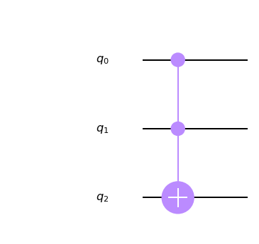
Because of the properties of \(\oplus\), the Toffoli is the inverse of itself. Thus, if we apply twice the Toffoli gate to the same 3 qubits, the working qubit will not change.

To consolidate those ideas, here is a Jupyter notebook that uses multiple-qubit gates:

Uncomputation

As we discussed in the previous session, we have seen that for calculating the AND of qubits \(|a\rangle\) and \(|b\rangle\), we need a working qubit to store \(|a \wedge b\rangle\).

It turns out that sometimes, to compute a generic function \(f(a, b)\), we may need even more working qubits to store intermediate results.

For example, imagine that you want to compute \(a \wedge b \wedge c\), the AND of three variables. You would need a qubit to compute \(a \wedge b\) and then another qubit to compute \((a \wedge b) \wedge c\).

Notice that we have very little interest in saving \(a \wedge b\). In general, it is a good idea to clean the results (i.e. to reverse the qubit to \(|0\rangle\)), because:

• We want to reuse resources
• It makes measurements more accurate (more qubits = more complex systems = harder measurements)

That process of cleaning is called uncomputation.

Because \((a \wedge b) \oplus (a \wedge b) = 0\), that is the inverse of the Toffoli gate is the Toffoli gate itself, then we may build the following circuit to calculate the AND of three qubits using uncomputation:

In the circuit above, we use an intermediary qubit \(|a \wedge b \rangle\) to help us achieve \(|a \wedge b \wedge c\rangle\), and then immediately clean it afterward. That way, the intermediary qubit goes back to \(|0\rangle\) and can be reused later if necessary.

The Qiskit code that implements the calculation of the AND of three qubits is provided bellow, building exactly the circuit we described: